Truly Understanding Quick Sort

Quick sort is one of the fastest practical sorting algorithms, but it is also interesting to study from a theoretical point of view.

1. It is very fast, both in practice and in theory. It can achieve a time complexity of Θ(n×log₂(n)) on average, which matches the best possible complexity in the worst case for comparison-based sorting algorithms.

2. It is an example of an in-place sorting algorithm. This means it does not use additional memory for the output or for processing, making it ideal in situations where memory is limited.

3. It is cache-friendly, making it very fast to execute on modern computers.

4. It is an example of a recursive algorithm, making it pedagogically important.

5. The algorithm is challenging to truly understand. When you finally get it, you will have a Eureka! moment.

6. It is historically important, as it was one of the first algorithms for sorting having a linear-logarithmic time complexity (on average).

How It Works - Overview

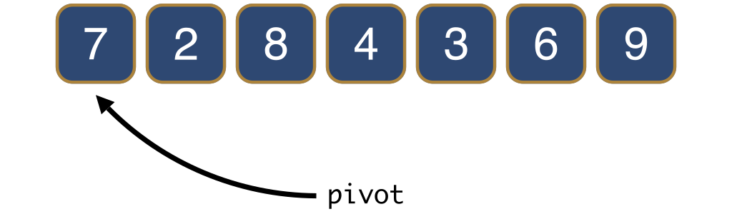
The main part of the quick sort algorithm is the so-called partitioning step. In order to partition an array, an element is arbitrarily chosen and called the pivot.

There are many strategies for choosing a pivot, each with its own advantages and disadvantages, but for simplicity let us simply choose the leftmost element.

Figure 1: Choose an arbitrary element and call it the pivot.

The partitioning sub-algorithm moves all elements smaller than the pivot to the left and all elements larger than the pivot to the right.

Figure 2: Move the elements smaller than the pivot to the left and the elements larger than the pivot to the right.

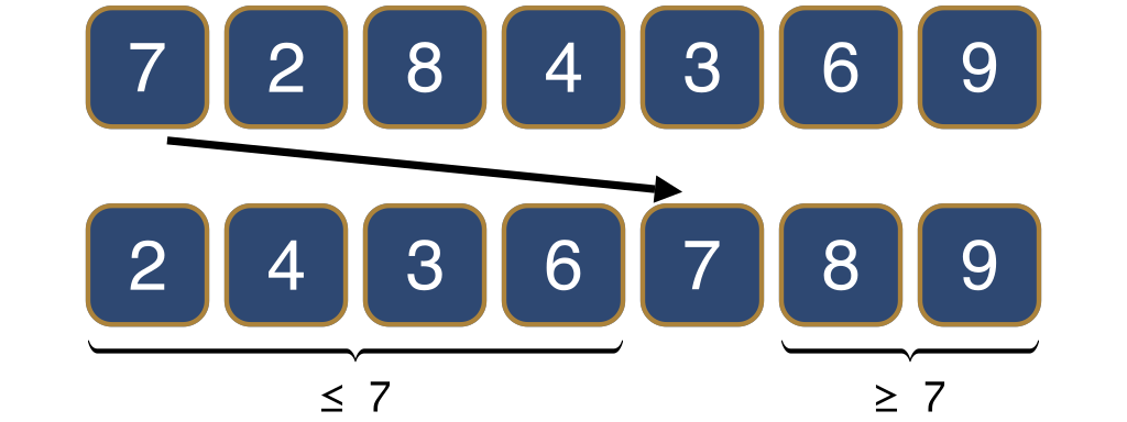
At this point, the order of the elements to either side of the pivot does not matter. What is important is that the elements to the left are smaller than the pivot and the elements to the right are larger.

Figure 3: The order of the elements to either side of the pivot does not matter at this point.

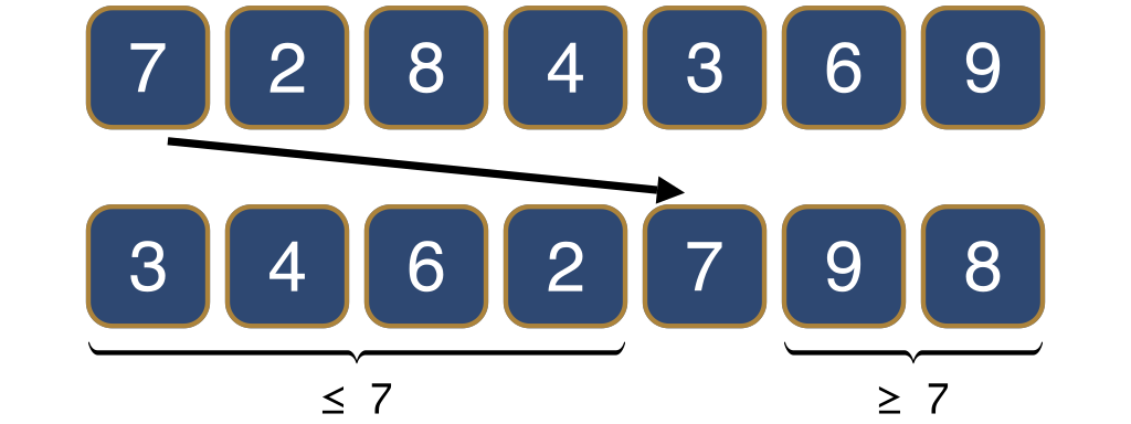
After partitioning, the pivot is in the same position as in the sorted array.

Figure 4: After partitioning, the pivot is in the same place as in the sorted array.

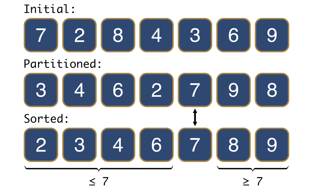
In order to obtain the final sorted array from the partitioned array, it is sufficient to sort what is to the left and to the right of pivot independently, using recursive calls.

In-place partitioning

The main difficulty in implementing quick-sort is to partition the array in-place, that is, without using additional storage space (or, at least, without using much additional storage space).

If we had additional space, we would walk the array one-by-one and save the elements smaller than the pivot into a second, auxiliary, array and the elements larger into a third array. At the end, we would find our partitioning by combining the smaller elements, the pivot, and the larger elements, in this order.

Figure 7: If we had additional space, partitioning would be very simple.

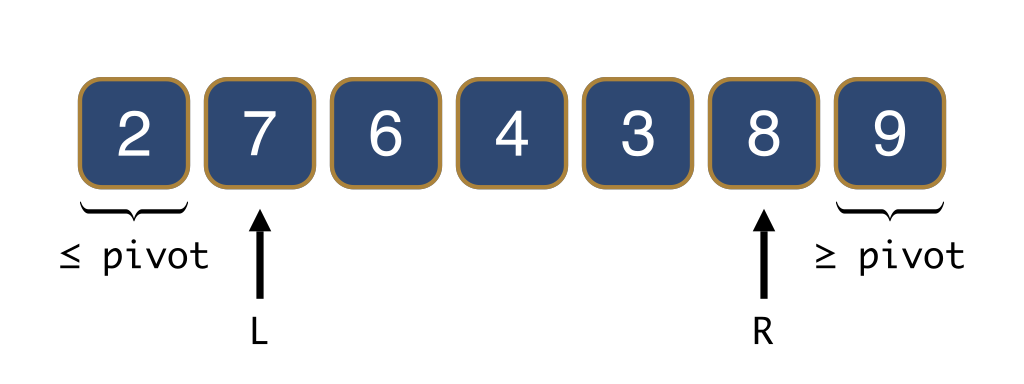
To achieve the partitioning in-place, i.e., without using additional storage, there are several strategies and I will show you the simplest one. We use two indices, L and R, that satisfy the property depicted in Figure 9.

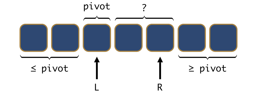
Figure 9: We maintain two indices, L and R, such that: (1) the pivot is at position L, (2) everything strictly to the left of L is smaller than the pivot, and (3) everything strictly to the right of R is larger than the pivot.

The elements other than the pivot between L and R, marked ? in the figure above, could each be either smaller, or larger than the pivot.

Initially, L points to the first element and R to the last element.

Figure 10: Initial state of the partitioning algorithm. All we know at this point is that the pivot is on the first position in the array.

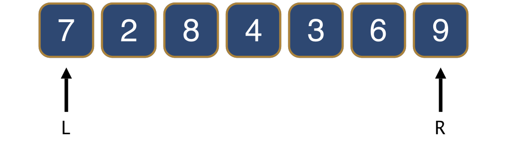
We now take steps that decrease R or increase L, in order to make the segment between L and R smaller and smaller, until L=R.

To make the segment smaller, we distinguish among three cases. The first case occurs when the element at position R is larger than the pivot. We simply move R one position towards the left. This ensures that to the right of R we only have elements larger than the pivot.

Figure 11: First case: the element at position R is greater than the pivot.

In the second case, the element at position L+1 is smaller than the pivot. We swap this smaller element with the pivot and increment L. This effectively moves the smaller element to the left of the [L,R] segment. This ensures that to the left of L there are only elements smaller than the pivot.

Figure 12: Second case: the element at position L + 1 is smaller than the pivot.

In the third and last case, the element at position L+1 is strictly greater than the pivot and the element at position R is smaller. It would be useful if it were the other way around, since then we would have been in the first two cases. Therefore, in this third case, we simply swap the elements at positions L+1 and R.

Figure 13: Third case: the element on position L + 1 is too large, but the element on position R is too small.

The segment [L,R] does not shrink in this third case. But the third case enables the following iterations to shrink the segment further by exercising Case I or Case II.

We iterate through one of the three cases until L becomes equal to R, at which point we are done: all elements smaller than the pivot are to the left and all elements larger than the pivot are to the right.

Figure 14: One of the three cases is taken until the array is fully partitioned.

The first case can be exercised at most n-1 times. This is because the index R moves towards the left. After more than n-1 steps, it would move beyond the beginning of the array.

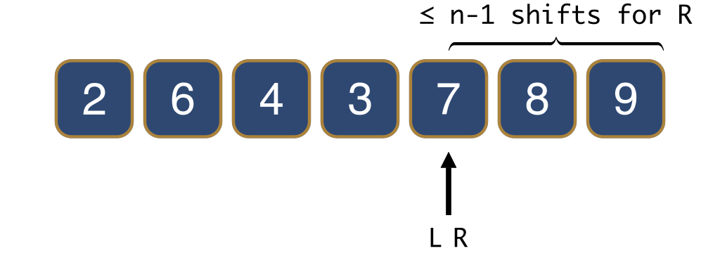
Figure 15: The index R is shifted leftwards at most n-1 times.

Using a similar argument, the second case is exercised at most n-1 times. [In fact, a more refined judgement would tell us that altogether, the first two cases cannot occur more than n-1 times.]

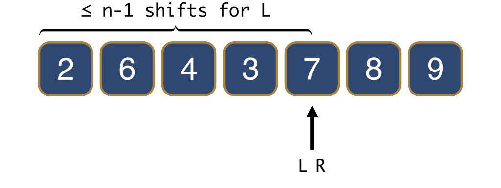
Figure 16: The index L is shifted rightwards at most n-1 times.

In the third case, we do not shift L, nor R. But the swap in the third case enables both a shift of R towards the left, and a shift of L towards the right in the following iterations. This means that it is followed by at least one first case and one second case (possibly more of each).

Figure 17: After the third case is exercised, both of the first two cases are enabled.

So the third case is exercised at most as many times as either of the first two cases. Overall, it is therefore also exercised at most n-1 times.

As each of the three cases takes constant time and occurs at most Θ(n) times, the time complexity of partitioning is Θ(n) × Θ(1) in the worst case, which amounts to Θ(n). Additionally, the partitioning algorithm works entirely in-place: there is no need for additional storage space, other than a few indices into the array.

How to Implement Quick Sort

Let us first implement a function for the partitioning algorithm. In the recursive calls to quick-sort, we will be needing to partition not just the initial array, but also sub-ranges of the initial array. The partition function therefore takes as input not only the array itself (int a[]), but also two indices, first and last, denoting the sub-range to partition. It partitions the range between first and last, inclusively, and returns the position of the pivot after partitioning.

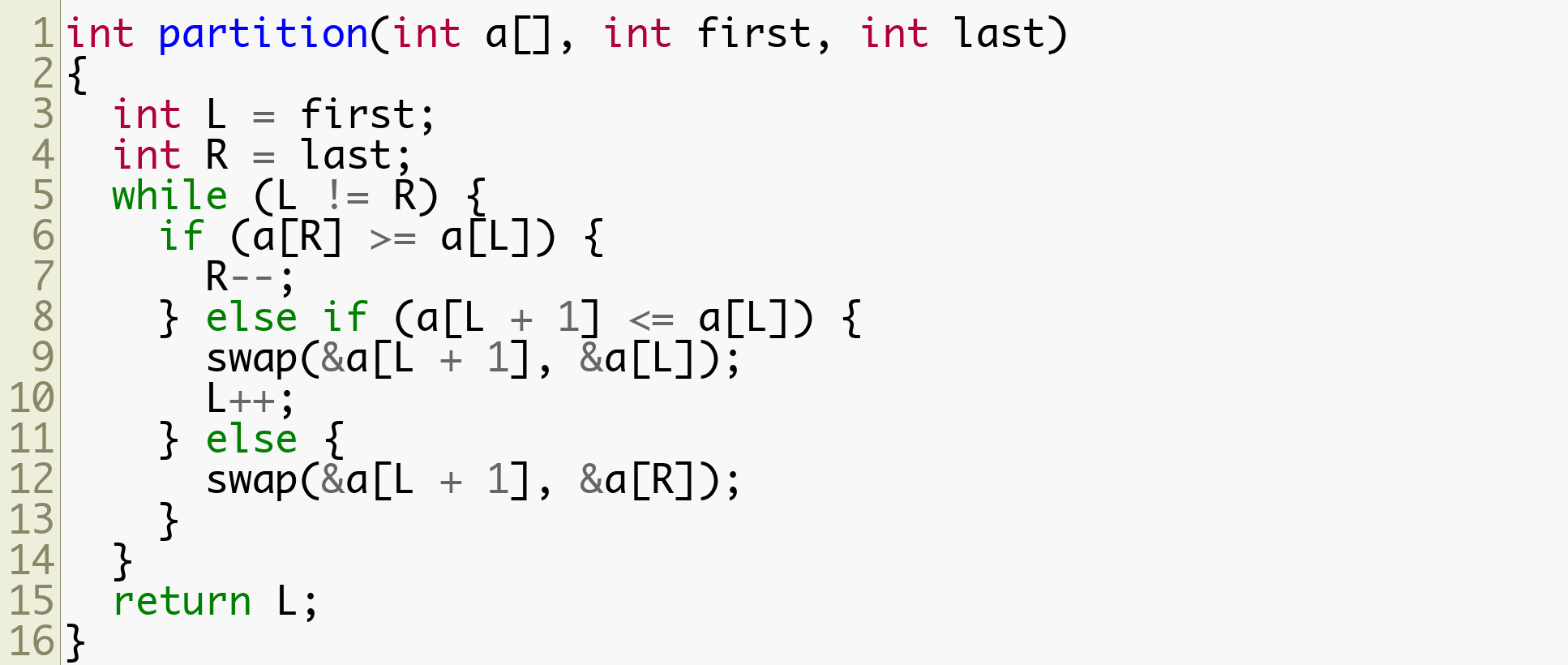
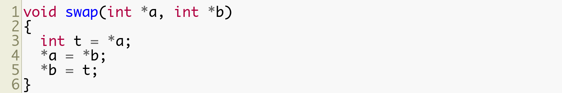
The implementation closely follows the discussion above: we repeatedly run one of the three cases, until the indices L and R become equal, and hence the range is partitioned. We return L, the position of the pivot after partitioning. We made use of the simple swap function, shown below.

Next, we will write a sort_range function, which does the main work of implementing the quick sort algorithm.

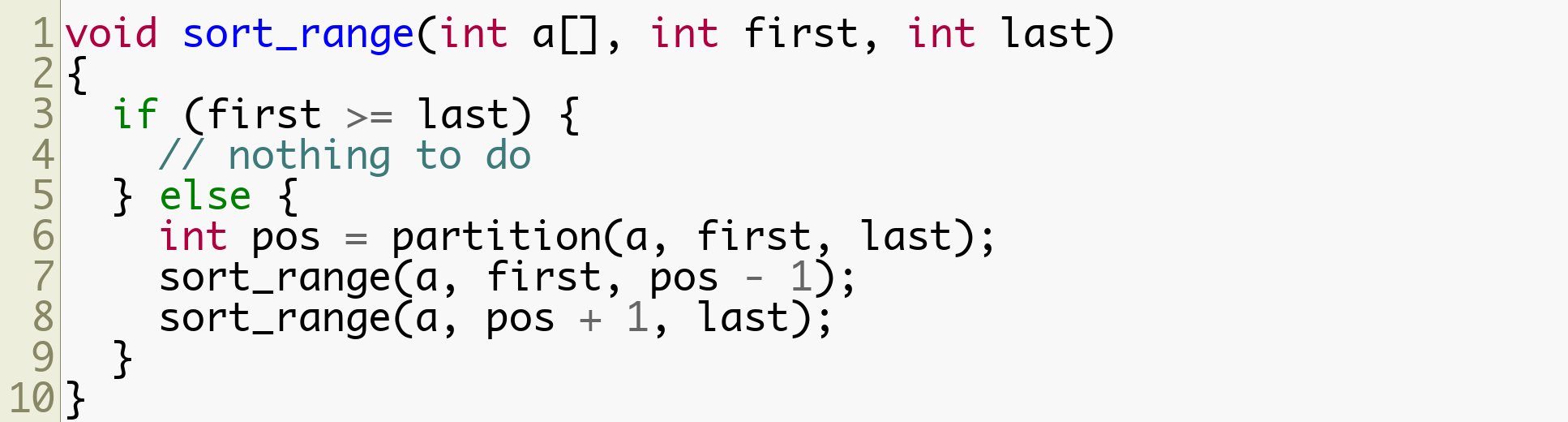
Its goal is to sort the range of the array a[] between the indices first and last, inclusively. In the base case (Line 4), the range is either empty, or consists of a single element. Therefore, there is no work to do. In the recursive case, we first partition the current range (Line 6). We save the position of the pivot after partitioning in the local variable pos; we need this information in the subsequent recursive calls. The pivot is in its final position after partitioning, so we do not need to do anything with it. Instead, we recursively sort the range to the left of the pivot (Line 7) and to the right of the pivot (Line 8).

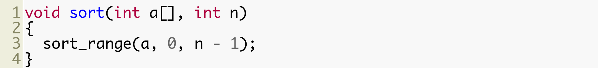
The function sort then simply calls sort_range on the entire array.

The Time Complexity

In the worst case, quick sort has a time complexity of Θ(n²), where n is the number of elements in the array. [This assumes that comparing and swapping elements of the array is a constant-time operation. This is usually a reasonable assumption, but it does not always hold. For example, sorting big integers or strings needs a more careful analysis of the running time.]

Worst-case time complexity. The worst case occurs when, say, the array is already sorted. Partitioning a sorted array of size n takes time θ(n), and the pivot remains on the first position (see Figure 18).

Figure 18: Partitioning a sorted array.

This causes sort_range to perform two unbalanced recursive calls: one on an empty range, and the other to a range having one element less than the current range. We end up calling sort_range on a range of size n, then n-1, then n-2, and so on, until reaching the base case on a range of size 1, as shown in Figure 19.

Figure 19: Visualising the recursive calls when the initial array is sorted.

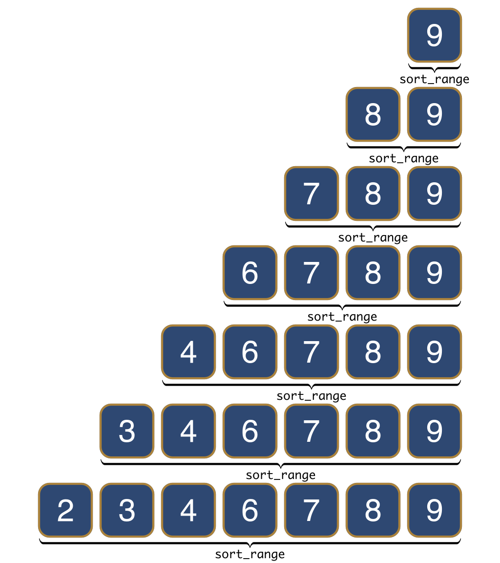
As each call to partition takes time linear in the size of the range, we end up with a time complexity in the worst case of Θ(n + (n-1) + (n-2) + … + 1), which is Θ(n²). On average however, assuming that the array given as input is a permutation of n distinct elements, and each permutation is equally likely, the running time is Θ(n×log₂(n)). I will now explain intuitively why this is the case.

If each permutation is equally likely to be given as input, the pivot is equally likely to end up on any given position after partitioning. Therefore, the expected position of the pivot is right in the middle of the array. This means that the two recursive calls work on an array of size roughly half that of the initial array.

Figure 20: The expected calls to sort_range for a random permutation.

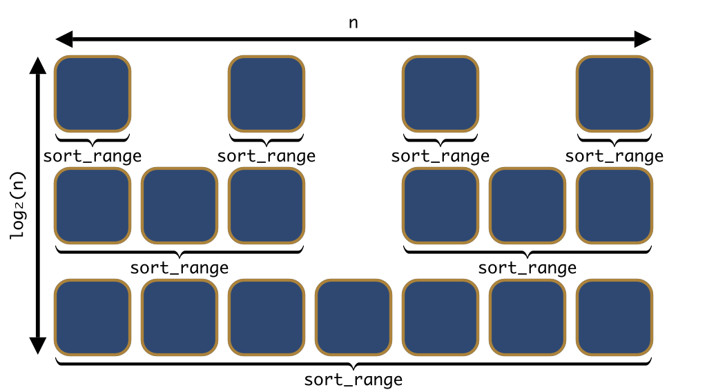
Each of the calls to sort_range makes a call to partition, which takes linear time. This means that each element in Figure 20 contributes Θ(1) towards the running time of the algorithm. Note how the elements sit on a matrix. There are n columns to the matrix. Because each line has ranges of size less than half that of the line below, there are about log₂(n) lines. So there are about n×log₂(n) elements overall, each contributing Θ(1) towards the running time, for a total running time of Θ(n×log₂(n)) in this case.

Best-case time complexity. What we have computed in the previous paragraph is actually the best-case time complexity of the algorithm. It is not necessarily the average-case time complexity. This is because, even if the expected position of the pivot is right in the middle of the array, the probability of the pivot ending up exactly in the middle at each recursive call is actually quite small.

Average-case time complexity. However, there is always a good chance that the pivot does not end up somewhere at the beginning or the end the of the array. For example, there is a very good (80%) chance that the pivot does not end up in the first 10%, nor the last 10% of the positions.

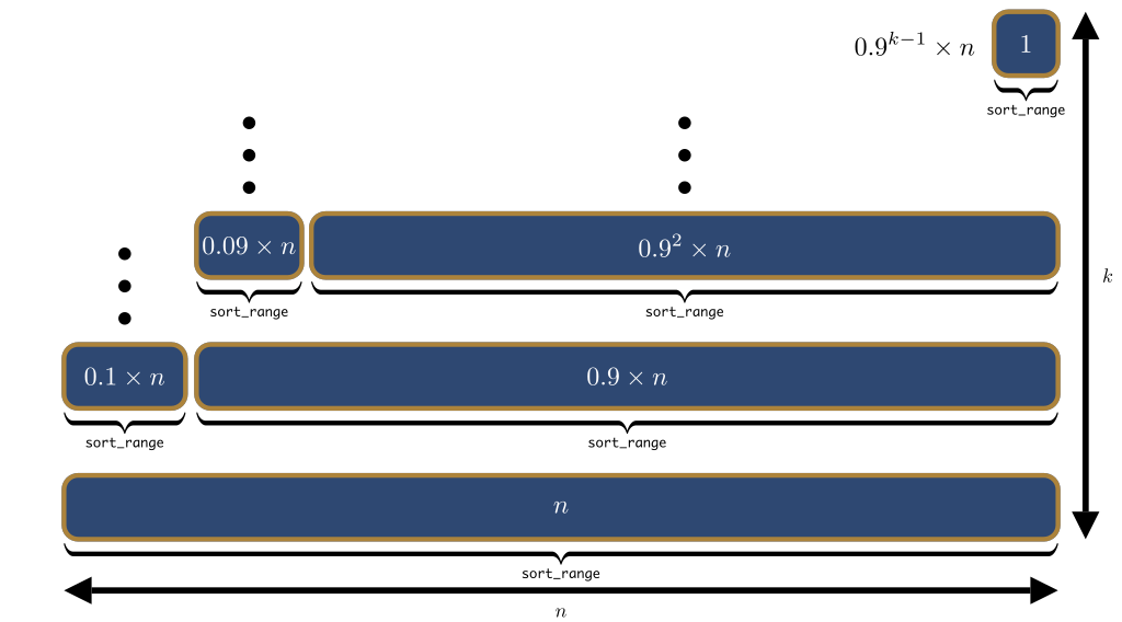
Figure 21: A depiction of the running time assuming a 1 to 9 split in each recursive call..

If the partition would split the array at a ratio of 1 to 9, as depicted in Figure 21, the running time would be Θ(n×k), where k is the smallest integer such that:

\(0.9^{k-1} \times n \leq 1.\)

We solve for k and obtain k to be roughly logᵢ(n), where i, the base of the logarithm, is 10/9. This gets us an overall complexity of Θ(n×logᵢ(n)). Under Θ-notation, the base of the logarithm is irrelevant, and therefore the running time is Θ(n×log₂(n)). The same line of reasoning can be used to show that the running time is Θ(n×log₂(n)) even when the split is 1 to 99, or 1 to 999, or any other constant ratio. This goes a long way to understanding the intuition behind the average-case time complexity, but it is not the entire story, because unbalanced splits are still somewhat likely to occur, at least some of the time.

Imagine we are unlucky at some point and end up with a 1 to n-2 partition. This unfavourable split will likely be offset in the following recursive calls, which will probably balance the partitions going forward, as depicted in Figure 22.

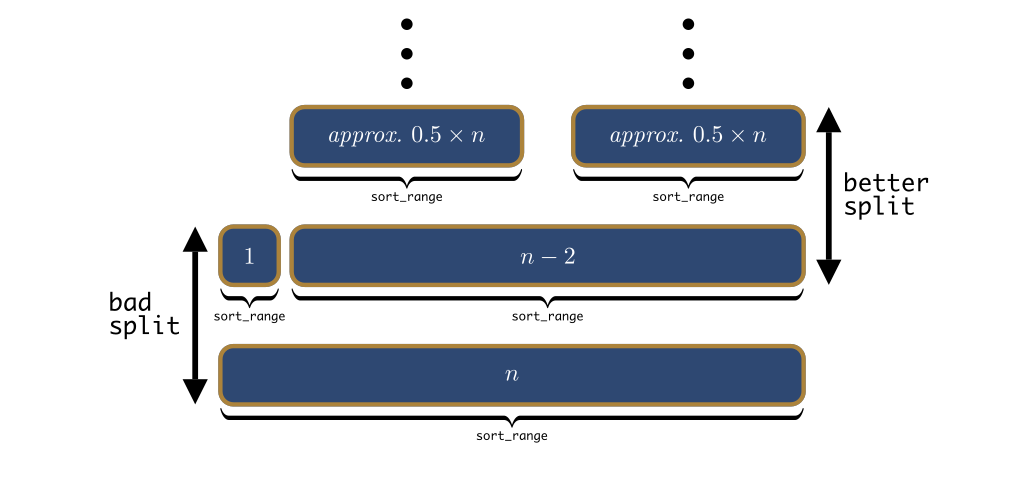
Figure 22: A depiction of an unlikely 1 to n-2 split, which is likely followed by a better, more balanced, split. Altogether, the two recursion levels depicted act similarly to two mediocre splits, and would still lead to a good time complexity.

In fact, it is highly unlikely to hit a Θ(n²) running time: we would need the pivot to end up within a constant number of items of the beginning (or the end) of the array, and we would need this to happen at just about every iteration. These cases are so unlikely, that they contribute essentially nothing to the average-case running time. Instead, the more balanced splits are much more likely to dominate the average-case running time. This explains intuitively why on average quick sort is Θ(n×log₂(n)). A formal proof is not terribly complicated either, and might make a future post.

There is also a simple technique to make the running time of the algorithm depend only on chance, not the input: just pick a pivot at random at each partition, any element in the range with the same probability. This improves the algorithm by making sure that no particular input can trigger the worst-case running time. The worst-case scenario still exists (now for every input) and it can occur, but the chance of it actually occurring is vanishingly small.